Understanding Continuous v. Discontinuous Limits.

Introduction

The concept of continuity and discontinuity of functions can be tricky to understand when learning about limits in your first Calculus class. It’s not only about figuring out what math method to use, but you have to understand what the conditions are that make a limit to fail to exist, and why.

A continuous function does not have any breaks in it, but continues in one smooth line or curve, no matter how complicated it looks.
A discontinuous function contains one or more points where the graph has a break, jump, hole, or vertical asymptote in it.

So, a continuous function f(x) is a function that varies continuously and has an output value (y) for every input value (x), while a discontinuous function is constructed in such a way that for certain input value(s) it renders the output invalid, and we say that the Limit Does Not Exist (DNE) at the given limit value.

Some examples that can make a function discontinuous are:

Rational functions: If the denominator is defined such that for a certain x it renders a zero value, because $f(x) = \\frac{a}{ x},x \\ne 0$ .
Even Root functions: because the function, $f(x) = \\sqrt[n]{x}$ for n = even , must satisfy $x \\ge 0$ . We don’t use imaginary numbers in this Calculus.
Trigonometric functions that are Rational functions: $f(x) = tan(\\theta) = \\frac{sin(\\theta)}{cos(\\theta)},\\; \\ cos(\\theta) \\ne 0$
Logarithmic functions: $f(x) = log(x), \\text{must have } x > 0$ . Remember, for Logs we can have, for example, x=0.000000000001, but NOT exactly at x = 0 or less.

The best way to start tackling a problem that asks you to determine if the function is continuous or discontinuous at a given limit $\\lim_{x \\to a} f(x)$ , is to first ask yourself “Does the function have any restrictions?” and if so, ask “What condition of the ones listed above, applies?” Once this is determined, what method should you use? 1) Can you do direct Substitution? 2) Solve it algebraically by using cancellations/eliminations? 3) Create a common factor by multiplying with a conjugate? This might seem overwhelming to determine, and there are other techniques to use as well. However, the best way is to take a step back and ‘observe’ how the problem ‘looks’. So, let’s solve two very similar looking functions to explore this problem, where the substitution and/or the algebraic methods apply.

Which is Continuous / Discontinuous ?

Both of these two functions below are very similar looking, and many AP high-school teachers and College professors often put similar questions on tests.
$$ \text{A) } \lim_{x \to 1}\frac{x^2 – 1}{ x + 1}\text{ } \text{ versus }\text{ } \text{ B) } \lim_{x \to 1} \frac{ x + 1} {x^2 – 1}$$

Find the Limit of A)
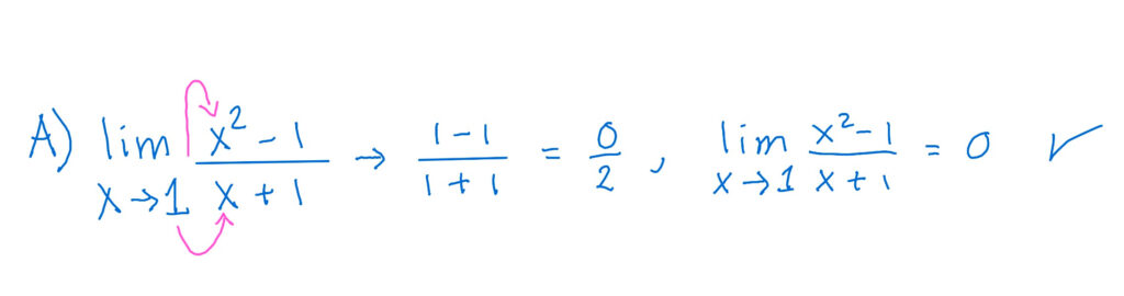
Let’s start with A). FIRST, Observe that there’s a denominator! What happens when you substitute 1 into x in the numerator and denominator? Is this mathematically ‘legal’? YES, because when popping in 1 for x we get 1+1 = 2 in the denominator, which is totally OK! So A) can be solved with straightforward substitution $(1^2-1)/(1+1) = 0$ (Figure 1).

fig2a — _{Figure 1. First try substituting in the limit for x, and see if the limit is valid. If it does, the limit is continuous at this point. Here we say that f(x) is continuous at (1,0), or just say continuous at x=1.}

Now, you may have a professor that requires you to cancel and eliminate where it is possible, which I consider should always be done. Therefore it’s important to recognize that the numerator is a Difference of Squares and factoring the numerator into $(x-1)(x+1)$ cancels the denominator. However, we still get the same answer (Figure 2).

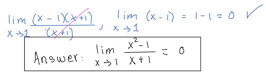
fig3a — _{Figure 2. Factoring the difference of squares in the numerator, cancels the denominator, using substituting in the limit for x, we get the same answer as in Figure 1.}

In summary, for a problem like this when you discover that the limit does not affect the constraint of the denominator, the best and easiest way to find the limit is to use the $substitution$ method, and just replace the function variable with the limit value. You can conclude that at x =1$, y=0, the limit value, and therefore f(x) is continuous at the point (1,0).

Find the Limit of B)
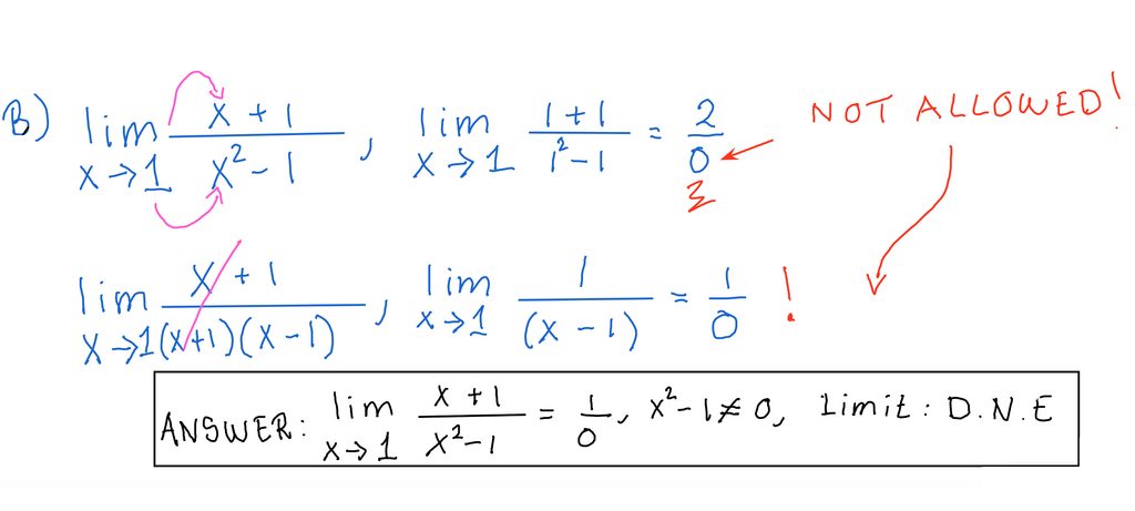
Let’s now look at the function on the right side B). As with the previous example, FIRST, observe that there is again a denominator! What happens now when you$substitute 1 into x in both the numerator and denominator? Is this mathematically ‘legal’? NO, because direct substitution produces division by zero! Therefore we must investigate further (Figure 3).

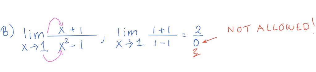
fig4a — _{Figure 3. Here when using the substitution method in the limit for x we get 0 in the denominator, therefore it looks like the limit Does Not Exist (D.N.E) at x=1, sp further investigation is needed.}

This situation definitely requires you to factor the Difference of Squares in the denominator to see if you can cancel and eliminate the restriction in the denominator for this limit. However, even though (x+1) in the denominator cancel with (x+1) in the numerator, we still are left with a restriction as ${x \\to 1}$ (Figure 4), and if we substitute in 1 for x we again get a zero in the denominator. Since with both methods we ended up with an undefined answer, we now can definitely conclude that the limit at x = 1 Does Not Exist (D.N.E).

fig5a — _{Figure 4. Factoring the difference of squares in the numerator, cancels the denominator, using substituting in the limit for x, we still get the same answer as in Figure 3. We can conclude that the limit at x = 1 Does Not Exist (D.N.E).}

What happens as x gets closer and closer to 1 for problem B) ?

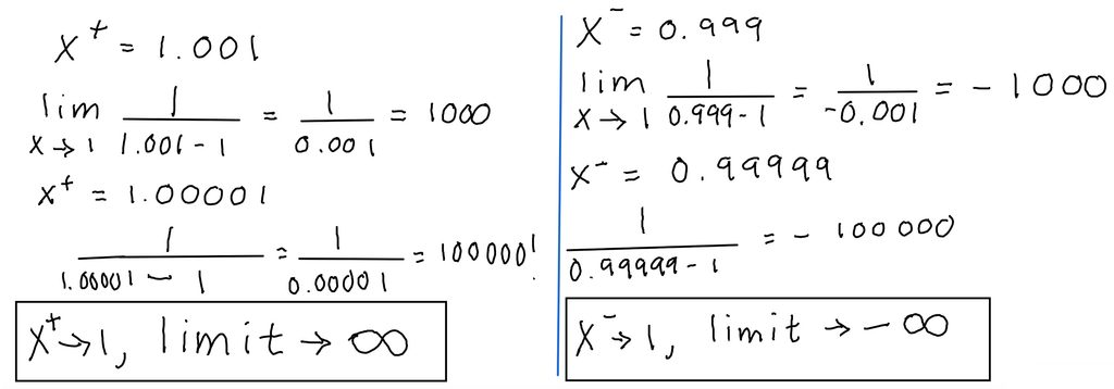
One crucial difference between Limit functions and regular functions is that with the Limits we investigate what happens as the independent variable approaches a specific value, not necessarily what happens exactly at this specific value ! For $\lim_{x \to 1}$ we can look at what happens as x gets closer and closer to the number 1, on either side of 1 !! This is what’s called Left and Right sided Limits, and denoted with a small + or – sign in the ‘exponent position’. When approaching from the Left we write: $x^{-}$ or $x\\to a^{-}$ and from the Right we write: $x^{+}$ or $x\to a^{+}$ for some real number a.

For example, if we let $x^{+} = 1.001, x^{+} = 1.0001$ , and then $x^{+} = 1.000001$ , what pattern emerges? As can be seen in the left column of figure 5, since the limit of f(x) becomes larger and larger and we can conclude that the limit approaches $+\\infty$ (positive infinity) as $x \\to 1$ . While if we let $x^{-} = 0.999, x^{-} = 0.9999,$ and then $x^{-} = 0.999999$ , the $\\lim f(x)$ becomes more and more negative$and we can conclude that the limit approaches $-\\infty$ (negative infinity) as $x \\to 1$ , figure 5.

fig6a — _{Figure 5. When substituting in values for x very close 1, we can determine what really happens to lim f(x) as x→1. In the left column, x+ is just slightly larger than 1, while on the right column x− is approaching 1 slightly below 1. Substituting in numbers closer and closer to 1 reveals a pattern that both sides get larger and larger, but one is negative the other is positive.}

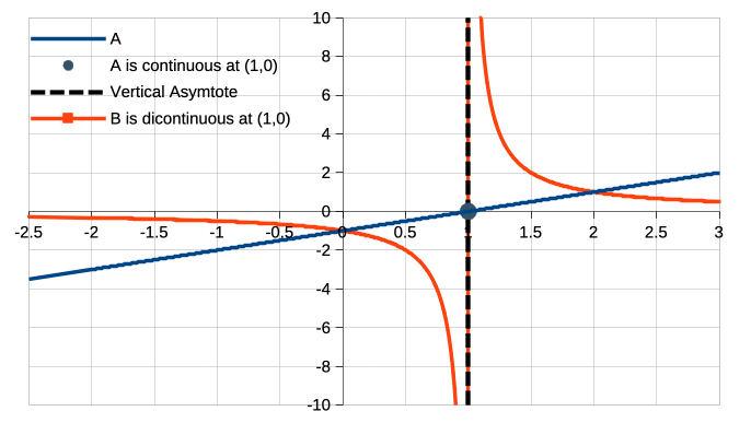
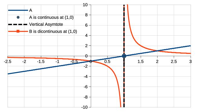
It is very useful to graph these functions, or any other function you are trying to solve and find if it is continuous and the limit exists at a specific point. In figure b we can clearly see that for problem A, we have a straight line and $\\lim_{x \\to 1} (x-1)$ exists at (1,0). But for problem B, the curves never reach (1,0), and the function is therefore discontinuous at this point. The red curves almost look like they would be two separate functions, but remember that they both belong to $f(x) = (x+1)/(x^{2} – 1)$, and exhibits a break that demonstrates its discontinuity.

fig9a — _{Figure 6. If you graph the functions of A (blue) and B (red), it becomes clear that A is in the shape of a straight line, and is continuous, while B veers off to infinity on both directions and is discontinuous because there is a break in this function.}

Conclusion of Limit Rules and Continuity

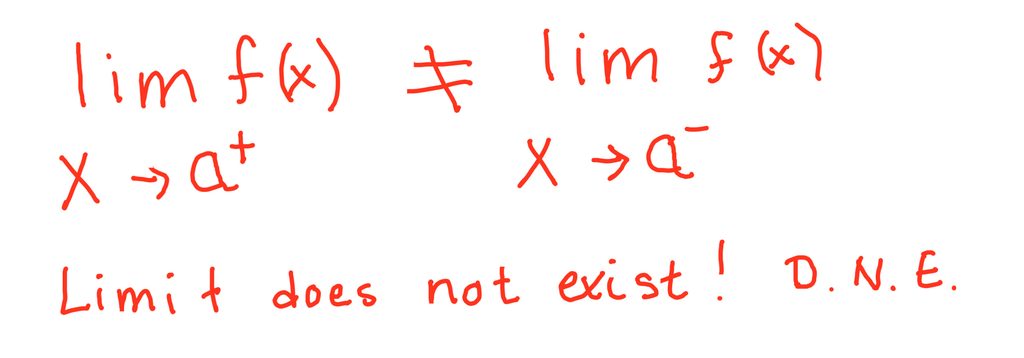
I always find that before presenting any complex mathematical theorems, it’s best to go over a few examples to see if a natural intuition of the rules emerges. For the two examples we just did, we may conclude that when the Left and Right side limits reach the same value, the Limit exists and f(x) is continuous at this specific point, otherwise it fails at the point in question and f(x) is therefore discontinuous (figure 6). This is almost true, the key word here is value; the function must reach a specific finite REAL number. In Calculus, continuity requires the limit to approach a specific finite value. So if you have a math limit problem where the left and right side both approach, for example, positive infinity, it will still be discontinuous due to the fact that infinity is not a real finite number, and of course when you think about it … can we reach infinity?

There are three conditions that must apply for a function to be continuous at a specific number and a more formal definition is:

A function f is continuous at a finite real number a if:

f(a) is defined, meaning a is in the domain of f.
Left limit and right limit equals the same number: $\\lim_{x\\to a^{-}}f(x) = A$ and $\\lim_{x\\to a^{-}}f(x) = A$
A common limit exists: $\\lim_{x\\to a}f(x) = f(a).$

fig7a — _{Figure 7. If the Left and Right side limits reach the same value, i.e a finite real number and the limit equals the function value, we say that the limit exists and f(x) is continuous. Otherwise it fails and it is discontinuous.}

Try it on your own !

On your own, examine the following limit problems below. In problem i I have just changed the limits of the same functions A) and B) and problem ii is very similar. But for problems iii and iv there’s some extra factoring to do first.

$$ (i) \text{ A) } \lim_{x \to -1} \frac{x^2 – 1}{ x + 1}\text{ } \text{ versus }\text{ } \text{ B) } \lim_{x \to -1} \frac{ x + 1} {x^2 – 1}$$

$$ (ii) \text{ A) } \lim_{x \to 3} \frac{x^2 – 9}{ x + 3}\text{ } \text{ versus }\text{ } \text{ B) } \lim_{x \to 3} \frac{ x + 3} {x^2 – 9}$$

$$ (iii) \text{ A) } \lim_{x \to 2} \frac{2x^2 – 8}{ x + 2}\text{ } \text{ versus }\text{ } \text{ B) } \lim_{x \to 2} \frac{ x + 2} {2x^2 – 8}$$

$$ (iv) \text{ A) } \lim_{x \to 4} \frac{x^2 – x + 12}{ x + 3}\text{ } \text{ versus }\text{ } \text{ B) } \lim_{x \to 4} \frac{ x + 3} {x^2 – x +12}$$

Give it a try ! Remember to check: 1) Does the denominator pose a restriction? 2) If so, what restriction applies? 3) Can you factor and eliminate?

When you have solved, check that all three conditions are satisfied to explain why f is continuous or not at the given limit as $x \to a$ so you can examine what happens at the (a,y) point. Note: the point may be there, whether or not the function is continuous at that point, as with part A). If we hadn’t removed it, the line would have a hole in it at (a,y). Also, if you’re familiar with any spreadsheet (Excel, Google Sheets, LibreOffice Calc), then graph these as well. A spreadsheet will require you to define an appropriate interval for your x values, for example [-3,3]. This will reveal where the function ‘breaks’ as the red curves show in Figure 6, which was made by LibreOffice Calc (LibreOffice is an open-source office suite and can be downloaded from https://www.libreoffice.org )Of course you can always use a fancy calculator like TI – 86 or higher, or use an online graphing software like Desmos ( https://www.desmos.com/calculator ) . However, I find that students understand better when their ‘fingers are more involved’, and best is of course to graph ‘by hand’.

I’d like to know how you did so do please leave a comment by simply clicking ‘comment’. Also, always try to solve as many problems as you can, especially the sections and concepts you are struggling with!

Good Luck and Thanks for reading!
——————–
Miss Liz
M.Sc. Physics.
B.S. Astrophysics.